Statistical Analysis
The user is advised to follow the modeling steps in the order suggested. Descriptive Statistics provides an overview of your data. In Preprocessing, the necessary datasets are prepared and tables can be edited. Under Modelling, the user can choose different model types, run the model and visualize and download results.
Contents
Descriptive Statistics
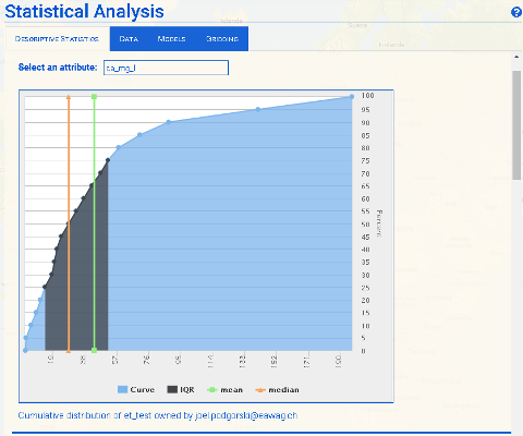
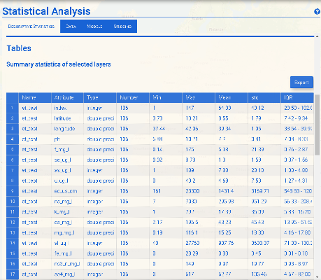
To view basic model statistics, select the model and go to Descriptive Statistics. You can view basic statistics for each variable either as a graph (Select an attribute) or as a table (Figure 1).
The cumulative distribution function (CDF) shows the number of datapoints below a respective threshold value. By clicking on the legend, you can visualize the dataset's mean, median and IQR (interquartile range), which indicates the middle 50% of the dataset.
The table contains the basic statistics for all attributes in the dataset.
| Name | Attribute | Type | Number | Min | Max | Mean | std | IQR |
|---|---|---|---|---|---|---|---|---|
| name of dataset | attribute name | data type | number of entries | minimum value | maximum value | mean value | standard deviation | interquartile range |
Data
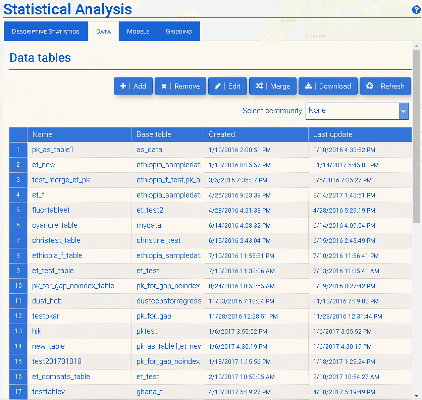
Before creating a statistical model, a modelling table must be prepared that includes all of the data to be used in modelling. This is done within the Data tab. Previously created modelling tables are also listed here.
Adding and editing a data table
First, choose the community you want to work in, if any, under Select Community. Otherwise, choose 'None'. Note that data tables will later be accessible only under community (or 'None') in which they were created.
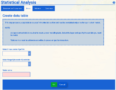
To create a new data table, click Add (Figure 1). Select the layer containing the data to be modeled, choose the target variable (Figure 3a) and specify a table name. The target variable will be the dependent variable of your model. The independent (predictor) variables will later get added to the table. Click OK to complete the process.
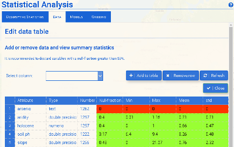
To edit a table, select it in the Data tab and click Edit (Figure 2). This will open a summary of the variables in the table to be included in your model (Figure 3b). Here you can add the independent variables to be used as predictors of the occurrence of groundwater contamination in your model. First, click on the drop-down menu Select column to display the list of all available layers. Once you have selected a variable, click Add. Some variables are more suitable than others, for example, due to their distribution of values. It is strongly recommended to remove any unsuitable variables (highlighted in red) before running your model. The color coding is defined as follows:
Red (not suitable)
- Null fraction (percentage of points of the dependent variable for which there are no values in the respective independent variable dataset) is > 50%, and/or
- Minimum value is the same as the maximum value (σ = 0), or
- Data type is non-numeric
Orange (not very suitable)
- 50% > null fraction >= 30%
Yellow (suitable)
- 30% > null fraction >= 20%
Green (very suitable)
- All other cases
To remove a variable, select it and click Remove.
Click Close once you have finished editing your table.
Models
The Models tab provides the functions/tools to develop a statistical model for the prediction of a geospatial parameter (e.g. geogenic groundwater contamination).
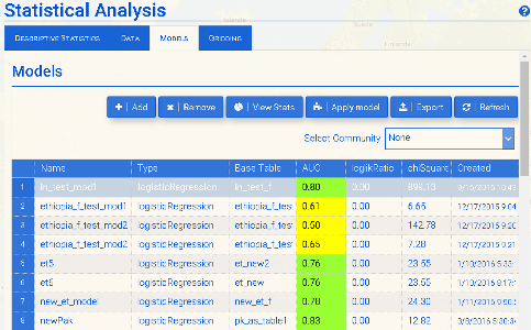
In the Models tab (Figure 4), you can add a new model (Add), view the statistics of an existing model table (View Stats), apply a model (Apply Model) or export the results of a model (Export). The (Refresh) button is available to update the list of models.
Logistic regression
The statistical modelling approach used by GAP is that of logistic regression. A logistic regression model gives the probability of a binary (0 or 1) target variable being "positive" (i.e. true or 1) for a linear combination of predictor variables. This is contained in a logistic function, which can be written as:: P(x) = frac {1}{1+e^{-(beta_0 + beta_1 x)}}
with P being probability, beta representing the coefficients of the regression and x being an independent variable. Note that multiple independent variables are possible.
The range of values of the logistic function are therefore from 0 to 1, which correspond probabilities of 0-100%.
You can learn more about logistic regression, for example, from this overview or this case-study example.
Create new model
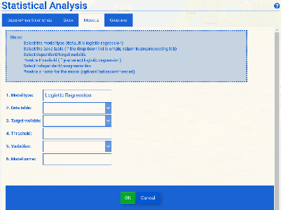
To create a new model, click Add, fill in the required information as indicated below and click Create when finished (Fig. 5). Note that if a community is selected under Select Community, the model will be created in this community. Select 'None' if you do not wish to create the model in a community.
1. The model can be run as either a logistic regression or a stepwise logistic regression. The latter approach calculates the model multiple times, removing poorly fitting independent variables with each step.
2. The base table should have been prepared in the Data section. (If the drop-down menu is empty, return to this section and create a data table.)
3. Select the target variable that you want your model to predict.
4. Threshold: Since logistic regression requires that the target variable is binary (0 or 1), the measured values of the dependent variable must be converted into binary format. A threshold is required to set the values that are less than or equal (<=) to this value to 0 and the values that are greater than (>) this value to 1. It often makes sense to set the threshold to the relevant contaminant concentration limit as determined by health organizations or local authorities. For example, current limits determined for drinking water by the World Health Organization (WHO) are 10 μg/l for arsenic and 1.5 mg/l for fluoride. Concentrations exceeding these values are considered hazardous to health.
5. For proxies, select the variables that are potentially suitable predictors (independent variables) for your target (dependent) variable. This selection is generally based on knowledge of the geochemical processes at work in the area of interest. However, other predictor variables suspected of playing a role can also be inserted into the model, which will ultimately show if a relationship exists for the data at hand.
6. Assign a model name.
The model is run after clicking Create, which adds a line to the Modelling tab containing the following information:
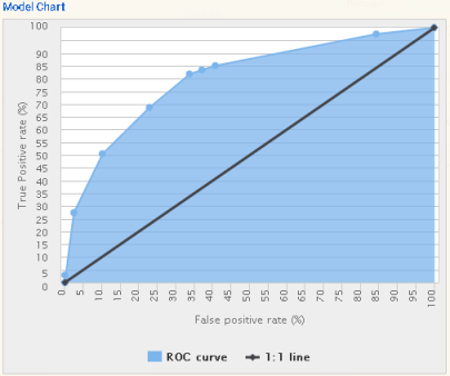
- AUC: area under curve, which is equivalent to the receiver operating characteristic (ROC) (see View Stats > Model Chart below for details)
- loglikRatio: -2 x logarithm of the ratio of the likelihood of the null model to the likelihood of the alternative (new) model. (A smaller value means a better fit of your model.)
- chiSquare: logistic regression chi-squared statistic, which is the difference in variance (unexplained dependent variable) between the null model and the alternative (new) model. (A larger chi-squared means a better fit of your model.)
View Stats
To view model statistics, select the model (Figure 4) and click View Stats.
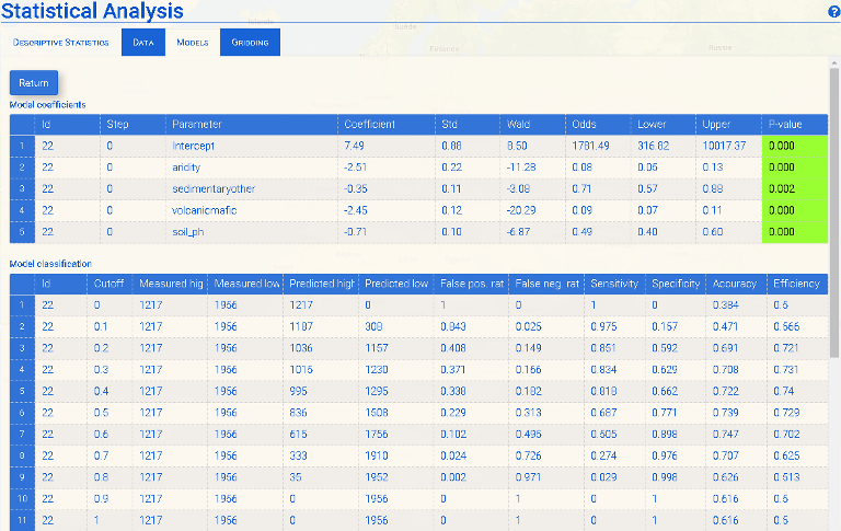
The Stats window contains three main sections: Model Coefficients, Model Classification and Model Chart.
Model Coefficients
The Model Coefficients table lists the following:
- Model ID - model number
- Step - step of a stepwise logistic regression
- Parameter - independent variable
- Coefficient - coefficient of the independent variable in the logistic function
- Std - standard deviation of the coefficient
- Wald - Wald statistic (coefficient/std), which is used to determine the p-value, which indicates the significance of the variable
- Odds - the multiplicative increase of the odds of the dependent variable being 1 for a unit increase of the independent variable
- Lower - lower bound of odds in the 95% confidence interval (using the coefficient minus two standard deviations)
- Upper - upper bound of odds in the 95% confidence interval (using the coefficient plus two standard deviations)
- P-value - probability that the relationship found between the independent variable and the dependent variable (the coefficient) is due to chance; also known as a z-test. Probabilities less than or equal to 0.05 (highlighted in green) are generally considered significant, which corresponds to a 95% confidence level that the relationship between the variables is real. Variables with a higher p-value are highlighted in red and should probably be removed from the model.
Model Classification
The Model Classification table displays the following:
- Model ID - model number
- Cutoff - value used with the model probabilities to set the model predictions to be either positive (high) or negative (low), i.e. 1 or 0, respectively
- Measured high - number of data measurements that are greater than the threshold set in the model, also known as "positives"
- Measured low - number of data measurements that are less than or equal to the threshold set in the model, also known as "negatives"
- Predicted high - number of positive (high) data measurements that are predicted by the model to be positive (high) at the given cutoff, also known as true positives (TP)
- Predicted low - number of negative (low) data measurements that are predicted by the model to be negative (low) at the given cutoff, also known as true negatives (TN)
- False positive - proportion of negative measurements (below threshold) incorrectly identified by the model as being positive (above threshold); equivalent to 1 - specificity
- False negative - proportion of positive measurements (above threshold) incorrectly identified by the model as being negative (below threshold); equivalent to 1 - sensitivity
- Sensitivity - proportion of true positives (high values), which is the proportion of positive measurements (above threshold) correctly identified by the model
- Specificity - proportion of true negatives (low values), which is the proportion of negative measurements (below threshold) correctly identified by the model
- Accuracy - proportion of all measurements (positive and negative) correctly identified by the model: (TP+TN)/(TP+TN+FP+FN).
- Efficiency - arithmetic mean of sensitivity and specificity
Note that the statistics presented here can be used to help determine the optimal cut-off value to use with the model. For example, the cut-off associated with the largest combination of sensitivity and specificity, or alternatively accuracy, could be selected.
Model Chart
A logistic regression can be evaluated by the trade-off between sensitivity (true positive rate) and specificity (true negative rate) for all possible cut-off levels. When plotted with 1 – specificity (false positives) on the x-axis and sensitivity on the y-axis, the area under the curve (AUC) provides an important indicator of the performance of the logistic regression (Fig. 6b). An AUC of 0.5 corresponds to a random selection (diagonal "1:1" line in Fig. 6b), whereas a model with a value of 1 perfectly predicts the observations. A logistic regression with an AUC greater than 0.7 is generally considered to be a good model that reasonably accurately depicts the data. AUC values greater than or equal to 0.7 are highlighted in the main Modelling window in green, whereas those less than 0.7 are highlighted in yellow.
Apply Model
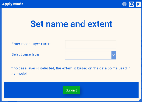
To generate a probability map based on a certain model, select the model and click 'Apply Model'. Then provide a name and select a layer to be used for calculating extent and resolution of probability map. You can also leave the latter option blank, then the model extent will be calculated based on the measurement points you provided.
Gridding
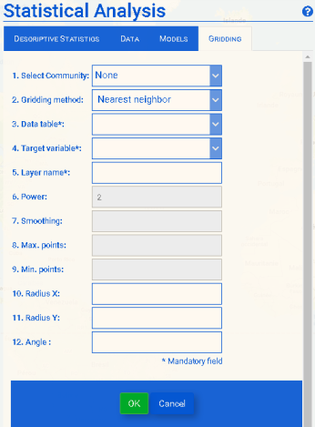
The Gridding function allows you to grid your point data using interpolation, which can produce a reasonably accurate map given a sufficient density of data points. Although not as sophisticated as logistic regression, found in the Models section, is simpler and easier to use and can be sufficient in some cases. The two main options to choose between are between the inverse distance and nearest neighbor algorithms. For more information, see the GDAL Grid Tutorial.
Inverse Distance The Inverse Distance method performs weighted average interpolation to a power (default 2). Optional parameters include:
- Smoothing - (default 0.0)
- Max. points - Maximum number of data points to use. Do not search for more points than this number. This is only used if search ellipse is set (both radii are non-zero). Zero means that all found points should be used. Default is 0.
- Min. points - Minimum number of data points to use. If less amount of points found the grid node considered empty and will be filled with NODATA marker. This is only used if search ellipse is set (both radii are non-zero). Default is 0.
- Radius X - The first radius (X axis if rotation angle is 0) of search ellipse. Set this parameter to zero to use whole point array. Default is 0.0.
- Radius Y - The second radius (Y axis if rotation angle is 0) of search ellipse. Set this parameter to zero to use whole point array. Default is 0.0.
- Angle - Angle of search ellipse rotation in degrees (counter clockwise, default 0.0).
Nearest Neighbor The Nearest Neighbor method simply takes the value of nearest point found in the grid node search ellipse and returns it as a result. The optional parameters are:
- Radius X - The first radius (X axis if rotation angle is 0) of search ellipse. Set this parameter to zero to use whole point array. Default is 0.0.
- Radius Y - The second radius (Y axis if rotation angle is 0) of search ellipse. Set this parameter to zero to use whole point array. Default is 0.0.
- Angle - Angle of search ellipse rotation in degrees (counter clockwise, default 0.0).
Both types of grids require the specification of a data table, target variable and layer name.
